This tutorial is based on the book Deep Learning with Pytorch and is mostly focused on the PyTorch API and Part I of the book (see also the Jupyter notebook). Refer to the book and its corresponding code on Github for more detail.

Overview

PyTorch is a library for Python programs that facilitates building deep learning projects. It emphasizes flexibility and allows deep learning models to be expressed in idiomatic Python. PyTorch operates in eager mode by default. That is, whenever an instruction involing PyTorch is executed by the Python interpreter, the corresponding operation is immediately carried out by the underlying C++ or CUDA implementation. PyTorch also provides a way to compile models of ahead of time through TorchScipt. Using TorchScript, PyTorch can serialize a model into a set of instructions that can be invoked independently from Python, such as with ONNX. This is similar to how Tensorflow 1.0 was built in that the user had to define a computational graph that they later executed.

import torch

torch.cuda.is_available()

True

Data

We need to convert each sample from our data into something PyTorch can actually handle: tensors or multidimensional arrays. In the context of deep learning, tensors refer to the generalization of vectors and matrices to an arbitrary number of dimensions. They are similar to Numpy arrays and can be indexed in the same way but offer the ability to perform computation on GPUs. All items in a tensor must be numbers of the same type; supported types are defined in torch.dtype with the default being torch.float32. Both Numpy arrays and PyTorch tensors are allocated as contiguous blocks of memory containing C numeric types as opposed to Python lists which are collections of Python objects individually allocated throughout memory (see figure 3.3 in the book). Memory footprint is managed by torch.Storage instances storing tensors in memory as 1d contiguous blocks, improving data locality and performance.

torch.save and torch.load operate using the pickle protocol and can be used to save and load tensors. For interoperability, hdf5 is also supported.

Images are usually stored in a volume (num images x num rows x num cols). Similarly, time series data are stored in a volume where one dimension corresponds a unit of time the data is stored in (t x num rows x num cols).

Neural networks take tensors as input and produce tensors as outputs. In fact, all operations within a neural network and during optimization are operations between tensors, and all parameters (for example, weights and biases) in a neural network are tensors.

a = torch.ones(3, 3, dtype=torch.int)
b = torch.ones(3, 3)

a[0,0]

tensor(1, dtype=torch.int32)

b.dtype

torch.float32

a.shape

torch.Size([3, 3])

We’ve constructed two 3x3 tensors of 1s and when added we should get a 3x3 tensor of 2s. Slicing and reshaping tensors can be done with torch.view. This avoids copying such that the view shares the same underlying data.

a + b

tensor([[2., 2., 2.],
        [2., 2., 2.],
        [2., 2., 2.]])

b.view(-1, 9)

tensor([[1., 1., 1., 1., 1., 1., 1., 1., 1.]])

We can add an extra dimension to a tensor using the None indexing or the unsqueeze function

a[None]

tensor([[[1, 1, 1],
         [1, 1, 1],
         [1, 1, 1]]], dtype=torch.int32)

a.unsqueeze(0).shape

torch.Size([1, 3, 3])

The tensor API has many operations in the torch module but can also be called as methods of a tensor object. For example, with unsqueeze above we called it as a method of tensor a but we can also call it through the torch module. There are a number of operations though that exist only as methods of the tensor object and they operate inplace; they’re identified by a trailing underscore.

torch.unsqueeze(a, 0)

tensor([[[1, 1, 1],
         [1, 1, 1],
         [1, 1, 1]]], dtype=torch.int32)

a.zero_()

tensor([[0, 0, 0],
        [0, 0, 0],
        [0, 0, 0]], dtype=torch.int32)

a

tensor([[0, 0, 0],
        [0, 0, 0],
        [0, 0, 0]], dtype=torch.int32)

Above, our tensors are stored on the CPU. We can also transfer or create them on the GPU

points_gpu = torch.tensor([[4.0, 1.0], [5.0, 3.0], [2.0, 1.0]], device='cuda')

b.to(device="cuda:0")

tensor([[1., 1., 1.],
        [1., 1., 1.],
        [1., 1., 1.]], device='cuda:0')

Now both b and points_gpu are in GPU RAM and we can start seeing performance optimizations with operations on the GPU. We can also go back and forth between Pytorch and Numpy. If we were to convert a PyTorch tensor stored on the GPU to numpy, it would make a copy over to CPU, however converting a tensor on CPU RAM to numpy comes at no cost since they both use the same underlying buffer for storage. It’s good to note that numpy arrays are stored as torch.float64 when converted so it’s usually best to convert to torch.float32 to avoid memory footprint.

import numpy as np

np_array = np.random.randn(2,2)

torch_from_np = torch.from_numpy(np_array)

torch_from_np.to(dtype=torch.float32)

tensor([[-1.4850, -0.8921],
        [-0.4044, -0.0816]])

torch_from_np.numpy()

array([[-1.48500536, -0.89214756],
       [-0.40442433, -0.08158075]])

We can also name each dimension within tensors so that that they are easier to keep track. For example if we have 2 4x4 images with 3 channels: RGB. Funtions accepting dimension arguments can now take names instead. It’s still an experimental feature so we won’t go too in depth

imgs = torch.randn(2, 3, 4, 4, names=["batch", "channels", "rows", "columns"])

/home/ubuntu/miniconda3/envs/pytorch_37/lib/python3.7/site-packages/ipykernel_launcher.py:1: UserWarning: Named tensors and all their associated APIs are an experimental feature and subject to change. Please do not use them for anything important until they are released as stable. (Triggered internally at  /opt/conda/conda-bld/pytorch_1609143291274/work/c10/core/TensorImpl.h:890.)
  """Entry point for launching an IPython kernel.

imgs.shape, imgs.names

(torch.Size([2, 3, 4, 4]), ('batch', 'channels', 'rows', 'columns'))

imgs.sum("batch")

tensor([[[-0.6343,  1.5833, -0.0329,  0.1315],
         [-1.7858,  1.7780, -0.3074, -0.9811],
         [ 0.0191, -1.0221, -1.0766,  1.0057],
         [ 2.2630,  0.5581, -0.8069,  1.1776]],

        [[ 0.4011,  0.6641,  1.8183,  0.6076],
         [ 1.2858,  2.3704, -0.4399,  1.4958],
         [ 0.2001,  1.7927,  2.6371,  2.9855],
         [-2.7196,  0.7211,  0.2021, -0.4641]],

        [[ 0.6448,  0.2991, -1.6020,  1.5254],
         [-0.1349,  0.6821,  0.4125, -2.0789],
         [-0.5938,  0.6197, -0.8342, -0.6182],
         [-1.7776, -0.5511, -1.2878,  0.1249]]],
       names=('channels', 'rows', 'columns'))

Datasets

This bridge between our custom data (in whatever format it might be) and a standardized PyTorch tensor is the Dataset class PyTorch provides in torch.utils.data. Simply put, it’s object that is required to implement two methods: __len__ and __getitem__. The former should return the number of items in the dataset; the latter should return the item, consisting of a sample and its corresponding label (an integer index).

from torchvision import datasets

cifar10 = datasets.CIFAR10(".", train=True, download=True)

Files already downloaded and verified

len(cifar10)

50000

img, label = cifar10[3]
img, label

(<PIL.Image.Image image mode=RGB size=32x32 at 0x7F465D7E0ED0>, 4)

DataLoader

DataLoader is another class provided under torch.utils.data that helps with shuffling and organizing data into minibatches.

• lets us sample data with various sampling strategies.
• implements __next__ so it can be iterated over and integrated directly in our training loop
• provides functionality to load data in parallel by spawning child processes in the background so that it’s ready and waiting for the training loop as soon as the loop can use it.

train_loader = torch.utils.data.DataLoader(cifar10, batch_size=64, shuffle=True)

train_loader

<torch.utils.data.dataloader.DataLoader at 0x7f465d7ea090>

Learning

%matplotlib inline
from matplotlib import pyplot as plt

Estimating parameters

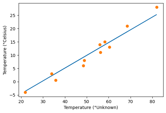
To get started, we’ll take some input temperature data in celcius t_c and some output data in unknown units t_u. We’ll assume there exists a linear relationship between the input and output and we’d like to learn their relationship by estimating paremeters of a linear model. That is we assume we can multiply t_u by some amount w and add a constant b to get t_c: t_c = w*t_u + b. We’ll estimate parameters w (weights) and b (biases) since they are not known. If we choose some values for w and b, how do we know how good of an estimate they are? We’ll use a loss function to measure the error between our predictions t_p and desired outputs t_c: (t_p - t_c)^2 (see section 5.3 for why we use this loss).

t_c = torch.tensor([0.5, 14.0, 15.0, 28.0, 11.0, 8.0, 3.0, -4.0, 6.0, 13.0, 21.0])
t_u = torch.tensor([35.7, 55.9, 58.2, 81.9, 56.3, 48.9, 33.9, 21.8, 48.4, 60.4, 68.4])

def model(t_u, w, b):
    return w * t_u + b

# initialize the parameters and invoke the model
w = torch.randn(())
b = torch.randn(())
t_p = model(t_u, w, b)
t_p

tensor([11.1664, 17.0082, 17.6733, 24.5272, 17.1238, 14.9838, 10.6459,  7.1467,
        14.8392, 18.3095, 20.6231])

def mse(t_p, t_c):
    """Loss function: mean squared error"""
    squared_diffs = (t_p - t_c)**2
    return squared_diffs.mean()

# calculate the loss function
mse(t_p, t_c)

tensor(47.0433)

We can keep randomly choosing values of w and b until we find values where the loss function is small enough but that’s inefficient. Instead we’ll use an iterative procedure to update our parameters called gradient descent. We’ll look at a small neighborhood around the current value of each parameter and find the direction where the loss is decreasing the most using the derivative. In a model with two or more parameters like the one we’re dealing with, we compute the individual derivatives of the loss with respect to each parameter and put them in a vector of derivatives: the gradient [dloss/dw, dloss/db]. In order to compute this vector of derivatives we’ll use the chain rule to compute dloss/dw = dloss/dmodel * dmodel/dw and dloss/db = dloss/dmodel * dmodel/db.

def dloss_dmodel(t_p, t_c):
    """Derivative of loss function (t_p - t_c)^2
    with respect to the output of the model t_p"""
    dsq_diffs = 2 * (t_p - t_c) / t_p.size(0)
    return dsq_diffs

def dmodel_dw(t_u, w, b):
    """Derivate of the model w * t_u + b
    with respect to w"""
    return t_u

def dmodel_db(t_u, w, b):
    """Derivate of the model w * t_u + b
    with respect to b"""
    return 1.0

def grad_fn(t_u, t_c, t_p, w, b):
    dloss_dtp = dloss_dmodel(t_p, t_c)
    dloss_dw = dloss_dtp * dmodel_dw(t_u, w, b)
    dloss_db = dloss_dtp * dmodel_db(t_u, w, b)
    return torch.stack([dloss_dw.sum(), dloss_db.sum()])

def training_loop(n_epochs, learning_rate, params, t_u, t_c):
    """Typically the training loop is implemented as a standard Python for loop. 
    Pytorch lightning gives more high level API on top of pytorch for training
    
    n_epochs: number of epochs - a training iteration that results in updating parameters for all training samples
    learning_rate: scaling factor that determines how much we update our weights by
    """
    for epoch in range(1, n_epochs + 1):
        w, b = params
        
        # forward pass
        t_p = model(t_u, w, b)
        loss = mse(t_p, t_c)
        # backward pass - backpropagating derivatives
        grad = grad_fn(t_u, t_c, t_p, w, b)
        # update parameters
        params = params - learning_rate * grad
        
        if epoch % 100 == 0:
            print('Epoch %d, Loss %f' % (epoch, float(loss))) # <3>
            
    return params

# simple normalization to prevent bias and weights from receiving different relative updates
t_un = 0.1*t_u
w_star, b_star = training_loop(n_epochs = 1000, learning_rate = 1e-2, 
                               params = torch.tensor([1.0, 0.0]),
                               t_u = t_un,  
                               t_c = t_c)
w_star, b_star

Epoch 100, Loss 22.148710
Epoch 200, Loss 16.608067
Epoch 300, Loss 12.664559
Epoch 400, Loss 9.857804
Epoch 500, Loss 7.860115
Epoch 600, Loss 6.438284
Epoch 700, Loss 5.426309
Epoch 800, Loss 4.706046
Epoch 900, Loss 4.193405
Epoch 1000, Loss 3.828538





(tensor(4.8021), tensor(-14.1031))

t_p = model(t_un, w_star, b_star)  # <1>

fig = plt.figure(dpi=100)
plt.xlabel("Temperature (°Unknown)")
plt.ylabel("Temperature (°Celsius)")
plt.plot(t_u.numpy(), t_p.detach().numpy()) # <2>
plt.plot(t_u.numpy(), t_c.numpy(), 'o')

[<matplotlib.lines.Line2D at 0x7f465203bf90>]

PyTorch Autograd

Above we have a simple model where it’s easy to write out the derivatives for the loss function and each parameter. However, as model complexity grows, this becomes unwieldy. The good news is PyTorch tensors can remember where they come from and can automatically provide the chain of derivatives from parent operations with respect to their inputs. PyTorch creates an autograd graph of operations that is traversed forward for the forward pass and backwards for the backwards pass to compute the gradients. We can re-write our learning procedure above by taking advantage of this autograd functionality.

# requires_grad=True tells PyTorch to track the entire family tree of tensors resulting from operations on params
# the value of the derivative will be automatically populated as a grad attribute of the params tensor
params = torch.tensor([1.0, 0.0], requires_grad=True)

params.grad

In order to populate the gradient, we start with a tensor with requires_grad set to True, get the model, compute the loss, then call backward on the loss tensor.

loss = mse(model(t_u, *params), t_c)
loss.backward()

loss, params.grad

(tensor(1763.8848, grad_fn=<MeanBackward0>), tensor([4517.2969,   82.6000]))

Now the grad attribute of params contains the derivatives of the loss with respect to each element of params

It’s important to note that calling backward causes gradients to accumulate at leaf nodes. In order to update parameters at each iteration of a training loop, they need to be zerod out explicitly after issuing updates. We can do this easily using the in-place zero_ method

def training_loop(n_epochs, learning_rate, params, t_u, t_c):
    for epoch in range(1, n_epochs + 1):
        if params.grad is not None:
            params.grad.zero_()
        
        t_p = model(t_u, *params) 
        loss = mse(t_p, t_c)
        loss.backward()
        
        with torch.no_grad():
            params -= learning_rate * params.grad

        if epoch % 100 == 0:
            print('Epoch %d, Loss %f' % (epoch, float(loss)))
            
    return params

Above we see the use of torch.no_grad. This code block tells PyTorch to update params inplace and not add an edge to the autograd graph. If we were using validation data to track training, computing the loss of the validation data would go in here as well since we wouldn’t want to build a graph for that. When using autograd we usually avoid inplace operations as done above because we might need the values we’d modify during the backward pass. Related functionality that can control whether we use autograd or not is torch.set_grad_enabled(bool) and is useful to distinguish between training and inference loops

w_star, b_star = training_loop(n_epochs = 1000, learning_rate = 1e-2, 
                               params = torch.tensor([1.0, 0.0], requires_grad=True),
                               t_u = t_un,  
                               t_c = t_c)
w_star, b_star

Epoch 100, Loss 22.148710
Epoch 200, Loss 16.608067
Epoch 300, Loss 12.664559
Epoch 400, Loss 9.857802
Epoch 500, Loss 7.860115
Epoch 600, Loss 6.438284
Epoch 700, Loss 5.426309
Epoch 800, Loss 4.706046
Epoch 900, Loss 4.193405
Epoch 1000, Loss 3.828538





(tensor(4.8021, grad_fn=<UnbindBackward>),
 tensor(-14.1031, grad_fn=<UnbindBackward>))

Gives same result as before when we manually differentiated everything!

Optimizers

import torch.optim as optim

Above we used vanilla gradient descent, but in practice there are better optimization techniques to deal with more complex models. A list of supported optimization algorithms are listed in torch.optim. Every optimizer constructor takes a list of parameters (aka PyTorch tensors, typically with requires_grad set to True) as the first input. All parameters passed to the optimizer are retained inside the optimizer object so the optimizer can update their values and access their grad attribute. Each optimizer exposes two methods: zero_grad and step. zero_grad zeroes the grad attribute of all the parameters passed to the optimizer upon construction. step updates the value of those parameters. We’ll use the optimizer package below to update our parameters automatically according to the chosen optimizer and a pre-defined learning rate. We can choose a more sophisticated optimizer with an adaptive learning rate such as Adam.

params = torch.tensor([1.0, 0.0], requires_grad=True)
optimizer = optim.Adam([params], lr=1e-1)

def training_loop(n_epochs, optimizer, params, t_u, t_c):
    for epoch in range(1, n_epochs + 1):
        t_p = model(t_u, *params)
        loss = mse(t_p, t_c)
        
        optimizer.zero_grad()
        loss.backward()
        optimizer.step()
        if epoch % 100 == 0:
            print('Epoch %d, Loss %f' % (epoch, float(loss)))
    return params

training_loop(
    n_epochs = 1000, 
    optimizer = optimizer,
    params = params,
    t_u = t_un,
    t_c = t_c)

Epoch 100, Loss 18.730587
Epoch 200, Loss 8.292550
Epoch 300, Loss 4.275753
Epoch 400, Loss 3.178962
Epoch 500, Loss 2.962302
Epoch 600, Loss 2.931170
Epoch 700, Loss 2.927909
Epoch 800, Loss 2.927659
Epoch 900, Loss 2.927646
Epoch 1000, Loss 2.927647





tensor([  5.3676, -17.3044], requires_grad=True)

The above parameters look an awful lot like those necessary for converting Celsius to Fahrenheit so we can conclude that the unknown unit of temperature is probably Fahrenheit. The exact values would be w=5.5556 and b=-17.7778

Torch.nn

torch.nn provides common neural network layers and other architectural components such as activation and loss functions. Neural network layers are called modules in PyTorch. A PyTorch module is a Python class deriving from the nn.Module base class. A module can have one or more Parameter instances as attributes, which are tensors whose values are optimized during the training process (think w and b in our linear model).

We’ll start by re-writing our linear model with torch.nn and then converting it to a neural network.

# split data into 80% training set and 20% validation set
n_samples = t_u.shape[0]
n_val = int(0.2 * n_samples)

shuffled_indices = torch.randperm(n_samples)

train_indices = shuffled_indices[:-n_val]
val_indices = shuffled_indices[-n_val:]

t_c.unsqueeze_(1)
t_u.unsqueeze_(1)

t_u_train = t_u[train_indices]
t_c_train = t_c[train_indices]

t_u_val = t_u[val_indices]
t_c_val = t_c[val_indices]

t_un_train = 0.1 * t_u_train
t_un_val = 0.1 * t_u_val

import torch.nn as nn

t_un_val.shape

torch.Size([2, 1])

PyTorch expects the 0th dimension in the tensor to be the number of examples in the batch, hence the unsqueeze op above; the size shows 2 examples, each having one input feature. PyTorch enforces batching because it improves performance if we send just enough compute to saturate the computational power of the GPU. It also helps with some models that calculate statistics over its input data - with a larger batch size, the statistics tend to become more meaningful.

Calling an instance of nn.Module with a set of arguments ends up calling a method named forward within its __call__ function. The forward method is what executes the forward computation, while __call__ does other rather important chores before and after calling forward. So, it is technically possible to call forward directly, and it will produce the same output as __call__, but this should not be done from user code. Now we’ll no longer need to initialize parameters w and b as we do above nor will we need our model and mse functions.

# arguments are number of input features, number of output features, and whether to include a bias (default True)
linear_model = nn.Linear(1, 1)

# forward pass
linear_model(t_un_val)

tensor([[0.8970],
        [1.8425]], grad_fn=<AddmmBackward>)

# linear model contains parameters w and b by default
optimizer = optim.Adam(linear_model.parameters(), lr=1e-1)
linear_model.weight, linear_model.bias

(Parameter containing:
 tensor([[0.4681]], requires_grad=True),
 Parameter containing:
 tensor([-0.7741], requires_grad=True))

def training_loop(n_epochs, optimizer, model, loss_fn, t_u_train, t_u_val,
                  t_c_train, t_c_val):
    for epoch in range(1, n_epochs + 1):
        t_p_train = model(t_u_train)
        loss_train = loss_fn(t_p_train, t_c_train)
        
        with torch.no_grad():
            t_p_val = model(t_u_val)
            loss_val = loss_fn(t_p_val, t_c_val)
        
        optimizer.zero_grad()
        loss_train.backward()
        optimizer.step()

        if epoch % 100 == 0:
            print(f"Epoch {epoch}, Training loss {loss_train.item():.4f},"
                  f" Validation loss {loss_val.item():.4f}")

training_loop(
    n_epochs = 1000, 
    optimizer = optimizer,
    model = linear_model,
    loss_fn = nn.MSELoss(), # using built in loss
    t_u_train = t_un_train,
    t_u_val = t_un_val, 
    t_c_train = t_c_train,
    t_c_val = t_c_val)

Epoch 100, Training loss 22.8464, Validation loss 25.7585
Epoch 200, Training loss 12.8624, Validation loss 15.5194
Epoch 300, Training loss 7.0491, Validation loss 8.7951
Epoch 400, Training loss 4.4477, Validation loss 5.1896
Epoch 500, Training loss 3.5104, Validation loss 3.4544
Epoch 600, Training loss 3.2351, Validation loss 2.6654
Epoch 700, Training loss 3.1687, Validation loss 2.3178
Epoch 800, Training loss 3.1557, Validation loss 2.1700
Epoch 900, Training loss 3.1535, Validation loss 2.1106
Epoch 1000, Training loss 3.1533, Validation loss 2.0885

# these are different than the previous training loop since we are now splitting our data
linear_model.weight, linear_model.bias

(Parameter containing:
 tensor([[5.2572]], requires_grad=True),
 Parameter containing:
 tensor([-16.7094], requires_grad=True))

Now we’ll replace our linear model with a simple neural network containing a linear module, followed by an activation function, feeding into another linear module (input layer, hidden layer, output layer). The activation functions allow us to learn non-linear relationships between parameters which seems overkill for our problem that was solved using a linear model but it makes it easy to introduce PyTorch concepts. In general, non-linearities allow the output function to have different slopes at different values and values to be concentrated in a certain range which are properties desirable for training.

from collections import OrderedDict

seq_model = nn.Sequential(OrderedDict([
        ("hidden", nn.Linear(1, 8)),
        ("activation", nn.Tanh()),
        ("output", nn.Linear(8, 1))
    ])
)
seq_model

Sequential(
  (hidden): Linear(in_features=1, out_features=8, bias=True)
  (activation): Tanh()
  (output): Linear(in_features=8, out_features=1, bias=True)
)

nn.Sequential gives a simple way to concatenate modules. We can specify the modules without the named OrderedDict as well but this makes it easier to track later on. We choose dimension 8 for the hidden layer arbitrarily - the dimension of the output layer however, must match so we can matrix multiply 1 x 8 x 8 x 1 -> 1 x 1. We can inspect our model and look at all of its parameters

for name, param in seq_model.named_parameters():
    print(name, param.numel(), param.shape)

hidden.weight 8 torch.Size([8, 1])
hidden.bias 8 torch.Size([8])
output.weight 8 torch.Size([1, 8])
output.bias 1 torch.Size([1])

# inspect output layer's initialized weights
seq_model.output.weight

Parameter containing:
tensor([[ 0.0730,  0.1601,  0.0291, -0.1636,  0.2347,  0.3223, -0.1034,  0.2086]],
       requires_grad=True)

optimizer = optim.Adam(seq_model.parameters(), lr=1e-2)

training_loop(
    n_epochs = 1000, 
    optimizer = optimizer,
    model = seq_model,
    loss_fn = nn.MSELoss(),
    t_u_train = t_un_train,
    t_u_val = t_un_val, 
    t_c_train = t_c_train,
    t_c_val = t_c_val)

Epoch 100, Training loss 85.7229, Validation loss 35.9689
Epoch 200, Training loss 37.0779, Validation loss 8.4389
Epoch 300, Training loss 21.5115, Validation loss 2.4983
Epoch 400, Training loss 12.5073, Validation loss 2.2060
Epoch 500, Training loss 7.5120, Validation loss 2.5850
Epoch 600, Training loss 4.2222, Validation loss 6.9852
Epoch 700, Training loss 2.6850, Validation loss 8.0673
Epoch 800, Training loss 1.9347, Validation loss 8.3633
Epoch 900, Training loss 1.5238, Validation loss 8.4401
Epoch 1000, Training loss 1.2923, Validation loss 8.4277

t_range = torch.arange(20., 90.).unsqueeze(1)

fig = plt.figure(dpi=100)
plt.xlabel("Fahrenheit")
plt.ylabel("Celsius")
# blue circles are the unknown temperature (well we sort of know it's fahrenheit)
plt.plot(t_u.numpy(), t_c.numpy(), 'o')
# do a forward pass of all temps 20-90 degrees, normalize by multiplying by 0.1 as we did during training
plt.plot(t_range.numpy(), seq_model(0.1 * t_range).detach().numpy(), 'c-')
# do a forward pass for inference and mark predicted points with an x
plt.plot(t_u.numpy(), seq_model(0.1 * t_u).detach().numpy(), 'kx')

[<matplotlib.lines.Line2D at 0x7f465176a450>]

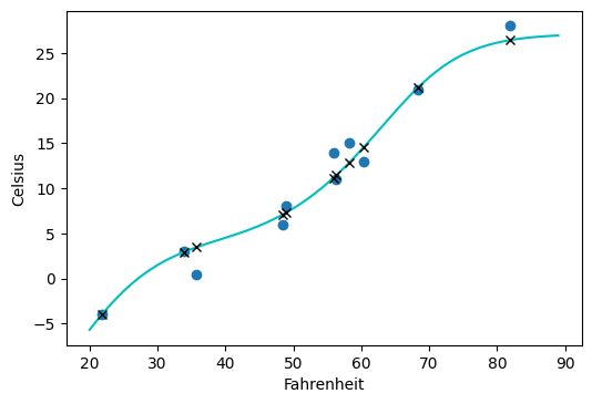
Compared to the linear model, the neural network overfits a bit with the s shaped curve above but it’s not too bad

When we want to build models that do more complex things than just applying one layer after another, we need to leave nn.Sequential for something that gives us added flexibility. PyTorch allows us to use any computation in our model by subclassing nn.Module. In order to subclass nn.Module, at a minimum we need to define a forward function that takes the inputs to the module and returns the output (PyTorch automatically takes care of the backward pass with autograd). Typically, our computation will use other modules—premade like convolutions or customized. Submodules must be top level attributes so that PyTorch can register them. We typically define submodules in the __init__ and assign them to self for use in the forward function. If a collection is needed we can use nn.ModuleList or nn.ModuleDict. Let’s convert the nn.Sequential model we defined to a subclass of nn.Module

class SubclassFunctionalModel(nn.Module):
    def __init__(self, n_hidden=8):
        super().__init__()
        self.n_hidden = n_hidden
        self.hidden = nn.Linear(1, n_hidden)
        self.output = nn.Linear(n_hidden, 1)
        
    def forward(self, input_):
        hidden_t = self.hidden(input_)
        activated_t = torch.tanh(hidden_t)
        output_t = self.output(activated_t)
        
        return output_t

Above we also make use of PyTorch’s functional API available in torch.nn.functional. We can replace all submodules that don’t have any parameters in favor of their functional counterparts. In this case we keep nn.Linear in as modules so that SubclassFunctionalModel will be able to manage their parameters during training. Since the torch.tanh activation function doesn’t have any paremeters, we can just use it directly through the functional API instead of having to intialize it first. We can now move our data and model to the GPU and train it there

device = (torch.device('cuda') if torch.cuda.is_available()
          else torch.device('cpu'))
print(f"Training on device {device}.")

Training on device cuda.

def training_loop(n_epochs, optimizer, model, loss_fn, t_u_train, t_u_val,
                  t_c_train, t_c_val):
    for epoch in range(1, n_epochs + 1):
        # same training loop as above, just moving data to GPU
        t_u_train = t_u_train.to(device=device)
        t_u_val = t_u_val.to(device=device)
        t_c_train = t_c_train.to(device=device)
        t_c_val = t_c_val.to(device=device)
        
        t_p_train = model(t_u_train)
        loss_train = loss_fn(t_p_train, t_c_train)
        
        with torch.no_grad():
            t_p_val = model(t_u_val)
            loss_val = loss_fn(t_p_val, t_c_val)
        
        optimizer.zero_grad()
        loss_train.backward()
        optimizer.step()

        if epoch % 100 == 0:
            print(f"Epoch {epoch}, Training loss {loss_train.item():.4f},"
                  f" Validation loss {loss_val.item():.4f}")

net = SubclassFunctionalModel().to(device=device)
# it is good practice to create the Optimizer after moving the parameters to the appropriate device
optimizer = optim.Adam(net.parameters(), lr=1e-2)

training_loop(
    n_epochs = 1000, 
    optimizer = optimizer,
    model = net,
    loss_fn = nn.MSELoss(), # using built in loss
    t_u_train = t_un_train,
    t_u_val = t_un_val, 
    t_c_train = t_c_train,
    t_c_val = t_c_val)

Epoch 100, Training loss 73.5727, Validation loss 29.7260
Epoch 200, Training loss 32.9347, Validation loss 5.9493
Epoch 300, Training loss 18.4127, Validation loss 2.8130
Epoch 400, Training loss 10.5109, Validation loss 2.7348
Epoch 500, Training loss 5.7748, Validation loss 5.7041
Epoch 600, Training loss 3.4524, Validation loss 6.7101
Epoch 700, Training loss 2.2990, Validation loss 7.6650
Epoch 800, Training loss 1.7077, Validation loss 8.2975
Epoch 900, Training loss 1.3894, Validation loss 8.3534
Epoch 1000, Training loss 1.2029, Validation loss 8.1462

Misc

torch.distributed and torch.nn.parallel offers functionality for distributed training

Both torchvision.models and Torch Hub provides pretrained models that anyone can use. Although torchvision is a library, Torch Hub is a repository for third party models that allows the community to share models they’ve built. User just have to include a hubconf.py in their repo and Torch Hub will see it.

from torchvision import models

dir(models)[:5]

['AlexNet', 'DenseNet', 'GoogLeNet', 'GoogLeNetOutputs', 'Inception3']