We’ll walk through the calculations needed for gradient-based learning in a simple network with one hidden layer.

These notes are taken from the video series from Welch Labs which I highly recommend watching if you’re trying to understand neural networks for the first time. Let’s jump in.

Suppose we have a training set $X \in \mathbb{R}^{n x m}$ with $n$ examples and $m$ features where $X_{ij}$ is the value for the $n^{th}$ example and $j^{th}$ feature. Assume that the data has already been normalized to the range $[0,1]$ (important for equally weighing features of different scales). Additionally, we have labels $y_i$ for each of the $n$ training examples and predictions $\hat{y_i}$ for $i \in [1,n]$.

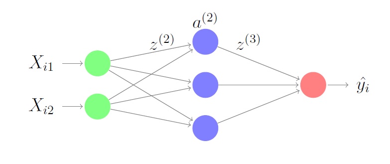
Our neural network will have an input layer of size $m$, a hidden layer of size $k$ and an output layer of size $1$. We will learn weights $W^{(1)} \in \mathbb{R}^{m x k}$ connecting the input layer to the hidden layer and $W^{(2)} \in \mathbb{R}^{k x 1}$ connecting the hidden layer to the output layer in order to minimize the error $J = \sum_{i=1}^n \frac{1}{2}(y_i - \hat{y_i})^2$. We will call the activity of our second layer $z^{(2)}=XW^{(1)}$. Once we apply the activity function to each element in the matrix $z^{(2)}$, we get $a^{(2)} = f(z^{(2)})$. Here, we’ll choose the activity function to be the sigmoid $f(z) = \frac{1}{1 + e^{-z}}$. Similarly, we do the same for the rest of the network and end up with the following equations:

\[z^{(2)}=XW^{(1)}\] \[a^{(2)} = f(z^{(2)})\] \[z^{(3)}= a^{(2)}W^{(2)}\] \[\hat{y} = f(z^{(3)})\] \[J = \sum_{i=1}^n \frac{1}{2}(y_i - \hat{y_i})^2\]

In order to minimize our loss function, we’ll use gradient descent which will involve taking the derivative of the loss function with respect to the weights. The key to doing so is repeatedly applying the chain rule since we’re dealing with function compositions. This is backpropagating the error to each weight.

\[\frac{\partial J}{\partial W^{(2)}} = -(y - \hat{y}) \frac{\partial \hat{y}}{\partial W^{(2)}}\] \[=-(y - \hat{y}) \frac{\partial \hat{y}}{\partial z^{(3)}} \frac{\partial z^{(3)}}{\partial W^{(2)}}\] \[=-(y - \hat{y}) f'(z^{(3)}) \frac{\partial z^{(3)}}{\partial W^{(2)}}\] \[=-(a^{(2)})^T (y - \hat{y}) f'(z^{(3)})\] \[\frac{\partial J}{\partial W^{(1)}} = -(y - \hat{y}) \frac{\partial \hat{y}}{\partial W^{(1)}}\] \[= -(y - \hat{y}) \frac{\partial \hat{y}}{\partial z^{(3)}} \frac{\partial z^{(3)}}{\partial W^{(1)}}\] \[= -(y - \hat{y}) f'(z^{(3)}) \frac{\partial z^{(3)}}{\partial a^{(2)}} \frac{\partial a^{(2)}}{\partial z^{(2)}} \frac{\partial z^{(2)}}{\partial W^{(1)}}\] \[= -X^T(y - \hat{y}) f'(z^{(3)}) (W^{(2)})^T f'(z^{(2)})\]

If we want to make a deeper neural network, we can just keep stacking these operations together. Now, in order to move in the direction to minimize our cost function, we’ll update our weights with some learning rate $\eta$:

\[W^{(i)} = W^{(i)} - \eta \frac{\partial J}{\partial W^{(i)}}\]

Once our weights stop changing very much, we can say our algorithm has converged.